How to implement bayer dithering for reducing an image to a lower bits per color format.

This article explains bayer dithering in a practical manner. If you really want a theoretical explanation of dithering, just read the Wikipedia articles on dither and ordered dithering.

For the purpose of this explanation we will be assuming our input graphics are stored in an RGB888 format. In other words, eight bits per color per pixel. This gives us an input value range of 0..255.

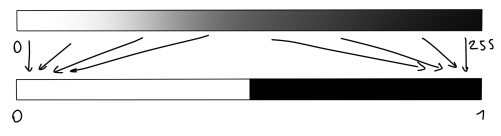
If you would be, for example, converting a grayscale image into a 1 bit black and white image, the simplest method would just do a >>= 7 operation, meaning values < 128 would become 0 and all values >= 128 would become 1. This generates a high contrast black and white image.

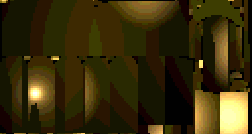
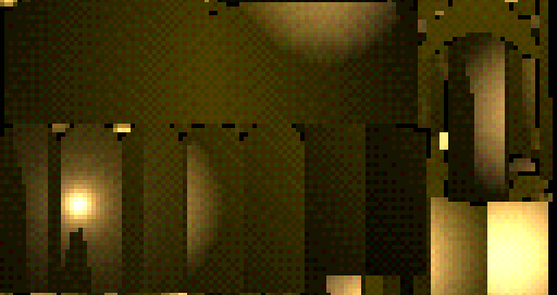
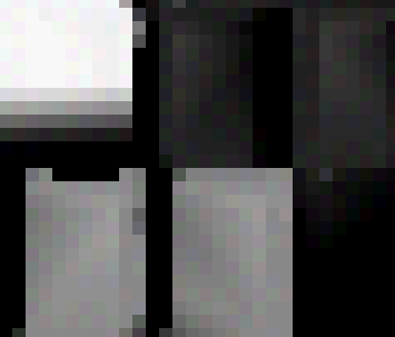
In a color conversion from RGB888 to RGB555, when simply doing a >>= 3 right shift, a lightmap used as example image ends up looking like this. The image contrast is enhanced here to better show the effect called banding.

Essentially, how dithering works, is that we simply add a pseudorandom value to every pixel before lowering the bits per color. This value is in the range equal to the loss of color precision, which causes a correctly proportioned amount of pixels to switch over to the next color value, resulting in a nice looking gradient.

In the case of a grayscale to 1bit conversion, we would add a value in range 1..255, and do a >>= 8 right shift operation to select all the values >= 256 as black.

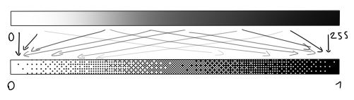
For a RGB888 to RGB555 conversion, we add a pseudorandom value to each pixel in the range 0..7 (where 7 is the masking value of the 3 lost bits), and do a >>= 3 right shift. The example image is contrast enhanced to clearly demonstrate the effect.

Note, that for the 1bit conversion I use a range starting at 1 instead of 0 and that I use 255 rather than the masking value of the lost bits (which would be 127). Due to the simplification of division by right shifting, the upper value is not exactly represented, and ends up being clipped off. The 1 bit conversion thus is a special case here. This behavior, however, is negligible, and is in any case preferred over having a value discontinuity anywhere else in the gradient caused by mathematically correct and slower division routines.

Now, to get a good quality dither, you cannot just use a random value. A common and simple method is to use a Bayer matrix as the source for your dither values. This is simply an infinitely repeating square lookup table, indexed by image coordinate.

A 2×2 Bayer matrix looks like this, and is constructed by starting anywhere, going to the furthest pixel from the starting point (which is a diagonal line), and then filling the remaining two pixels by the same logic.

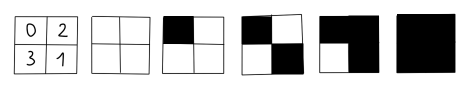
Essentially, the numbers represent the order in which pixels will advance to the next color value depending on the value level. Imagine converting from a set of 2 by 2 pixel solid gray images in range 0..4 (so, a total of 5 shades) to the 1 bit range 0..1. Using the above matrix, an image with value 0 would be the leftmost non-filled, value 4 would be the rightmost filled result. The gray 2×2 pixel images with the remaining in-between values, would be one of the three in-between results respectively. A large 50% gray image would become the recognizable checkerboard pixel pattern.

The minimum and maximum values are decided by the required range for the pseudorandom number as previously explained, that is, the masking value of the lost bits. To increase the maximum value, a larger matrix can be constructed by following the same pattern in a recursive manner.

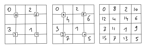
The same result can be obtained by duplicating the 2×2 matrix into a 4×4 matrix, multiplying all the values by 4, and adding the top-left value 0 from the original marix to the top-left 2×2 block, adding the original bottom-right value 1 to the bottom-right 2×2 block, and so on. This scales easily to generate much larger matrices. Practically, you’ll only need to go up to 16×16 to have a 0..255 matrix (for which you can just replace the 0 value by 1 to get the right initial value when using it to convert into 1 bit.)

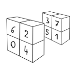
If you want to do some real fancy stuff, you could even follow the same patterns to generate a 3d bayer matrix. This can prove to be useful for procedurally generated 3d content using volumetric textures.

For converting RGB888 to RGB555, however, we need the highest value to be 7. Increasing the matrix size brings us from 3 straight to 15. To get to 7, simply >>= 2 right shift the matrix.

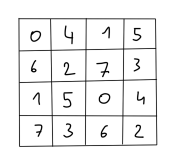
This results in a matrix where the bottom two 2×2 blocks are the flipped over version of the top two 2×2 blocks.

The basic formula used in the example is OUT = (IN + Bayer[x & 7][y & 7]) >> 3, where IN is in range 0..255 and OUT is in range 0..32 (calculated by (255 + 7) >> 3). As previously stated, the top value needs to be clipped off, so that the resulting range is 0..31, in order to fit into the 5 bits of the color channel.

While this provides a pretty good result already, we can slightly improve the quality by using a separate matrix for the different color channel. A simple method is to simply use a negative X coordinate for the Bayer matrix of the Red channel, and a negative Y coordinate for the Bayer matrix of the Blue channel (and optionally use the negative of both coordinates for the Alpha channel). This separation of color channels results in a perceived smoother transition. Example image is enhanced in contrast to better show the effect. Notice an improved reduction of banding in the bright light in the bottom left, compared to the previous dithered image.

Here’s a side-by-side comparison of the full image, without contrast enhancement, to show the actual visual result. Leftmost is the banded conversion, center is the first version of the dithering, rightmost is dithering with separation of color channels.

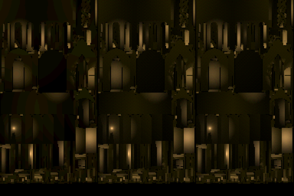
One side effect, however, of separating the color channel, is that this causes pure gray colors to lose their color purity. This is generally not much of an issue, as some colorization noise does have a certain artistic value to it. And you should probably not be using color textures if you require pure grayscale.

As a side note, the example here is using a lightmap texture which is in linear color space. If you were to convert a regular photographic image, which is usually in sRGB color space, to a 1 bit grayscale color depth, the image would first need to be converted into linear color space. A dithered gradient is in linear color space, as the display is only displaying pure black and white.

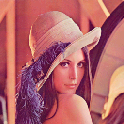
A post about image processing would not be complete, however, without the classic Lenna image. So here’s an RGB555 conversion of a 256×256 Lenna source image using bayer matrix dithering with separated color channels.